Spectral Averaging
Cycles are not static, so what?
Most cycle analysts have seen the moment-to-moment fluctuations, often referred to as shifts in the length and phase of a cycle, which are common in continuous measurements of a supposedly steady spectrum of financial records. But wait, we should know that cycles are not static in real life. We can see these variations in size and phase for each cycle length in the updated spectrogram after a new data point/bar is added to the data set. Although small variations are certainly no cause for concern, we should remember that we do not live in an ideal, noise-free world, but we are always looking for ways to reduce the phase shifts and variations in dominant cycles.
Therefore, instead of additional smoothing of the input data, we will apply averaging to the received cycle spectrum. The basic idea of averaging to reduce spectral noise is the same as averaging - or smoothing - the input signal. However, touching the raw input signal with the averaging reduces data accuracy and results in a delay of the signal. This is not what we need, especially because the end of the data set - the current time - is of the utmost importance when working with cycles for financial time series data. Therefore, averaging the input and adding a delay to our series of interest is a bad idea for cycle analysis in data sets where the most recent current data points are more important than data points from long ago.
Dont smooth the input - average the spectrum!
Averaging a spectrum can reduce fluctuations in cycle measurements, making it an important part of spectrum measurements without changing the input signal or adding delay.
Spectral averaging offers a different approach and is a kind of ensemble averaging, meaning that the "sample" and "average" are both cycle spectra. The "average" spectrum is obtained by averaging the "sample" spectra. However, due to the nature of the spectra, this is not as simple as this. If you apply a discrete Fourier transform routine to a set of real-world samples to find a spectrum, the output is a set of complex numbers representing the magnitude and phase of that spectrum. Calculating an average spectrum involves averaging over common frequencies in several spectra.
Spectral averaging eliminates the effect of phase noise.
The size of the spectrum is independent of time shifts in the input signal, but the phase can change with each data set. By averaging the power spectra and taking the square root of the result, we eliminate the effect of phase variation. Reducing the noise variance helps us to distinguish small real cycles from the largest noisy peaks.
The result of spectral averaging is an estimate of the spectrum containing the same amount of energy as the source. Although the noise energy is preserved, the variance (noise fluctuation) in the spectrum is reduced. This reduction can help us reduce the detection of "false cycles" that are the result of single, one-time "noise" peaks. Lets illustrate the concept of spectral averaging with a simple example.
This method is a derivative of the so-called Bartlett method, if no other window than a rectangular window is applied to the data sections.
Cycle detection example
We use a constructed, simplified data-set which consists of 2 cycles, noise and different trends. The two cycles have a length of 45 and 80 days:

Raw input signal consisting of cycles, noise and trends
Let us have a look at the different spectrogram results without (1) and with (2) spectral averaging. The first diagram shows the basic amplitude spectrum of the signal without spectral averaging.
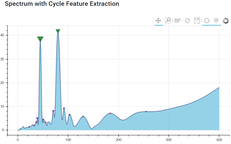
Chart 1: Cycle spectrum without spectrum averaging
It clearly shows the cycles with a amplitude peak at 45 and 80 days, but you can identify lower peaks in the spectrum that have nothing in common with real cycles of the original dataset. These smaller amplitude peaks are "false cycle" - noise only. We want to avoid using these cycles in cycle forecasting models.
Since it is important to identify and separate peaks based on noise - we will see if the method of averaging in the spectrum offers some added value. The next diagram uses the same input signal, but runs not just once to generate the spectrum, but several spectra to form the spectral average. In our case, the window only changes the beginning of the series and always uses the same end point for each spectrum.
This ensures that we have overlapping windows, always using the last available closer/bar and changing only the beginning of the series.
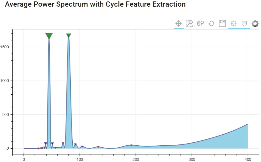
Chart 2: Cycle spectrum with spectrum averaging
The result illustrates that the peak values for 45 and 80 days are still present. But now the "noise" level has become much lower, and due to the averaging of the spectral window analysis, we have a lower number of "false cycle peaks". This will help us distinguish between important and unimportant cycles for future cycle prediction modeling techniques.
References:
- (2008) "The Spectral Analysis of Random Signals", in: Digital Signal Processing. Signals and Communication Technology. Springer, London. https://doi.org/10.1007/978-1-84800-119-0_7
- Oppenheim and Schafer (2009): "Discrete-Time Signal Processing", Chapter 10, Prentice Hall, 3rd edition.
- Bartlett (1950): "PERIODOGRAM ANALYSIS AND CONTINUOUS SPECTRA", Biometrika, Volume 37, Issue 1-2, June 1950, Pages 1–16, https://doi.org/10.1093/biomet/37.1-2.1
- Wikipedia: "Bartlett Method", https://en.wikipedia.org/wiki/Bartlett%27s_method
- Shearman (2018): "Take Control of Noise with Spectral Averaging", https://www.dsprelated.com/showarticle/1159.php