How to put cycle analysis into practice
Cycles are important. Cycles surround us and influence our daily lives. Many events are cyclical in motion. There is the ebb and the flow of waves and the inhaling and exhaling of humans.
Our daily work schedule is determined by the day and night cycles that come with the rotation of the Earth around its own axis. The orbit of the Moon around the Earth causes the tides of the oceans.
Gardeners have long understood the advantages of working with cycles to ensure successful germination of seeds and high-quality harvest. They work in harmony with the cycles to attain the best results, the best crops.
These are just a few cycles with recurring, dominant conditions that affect all living beings on Earth.
So if we are able to recognize the current dominant cycle, we are able to project and predict behavior into the future.
Let us start with a simple example to illustrate the power of today’s digital signal processing.
Figure 1 shows the daily outdoor temperature in Hamburg, Germany (blue). This raw data was fed into a digital signal processor to derive the current underlying dominant cycle and project this cycle into the future (purple).
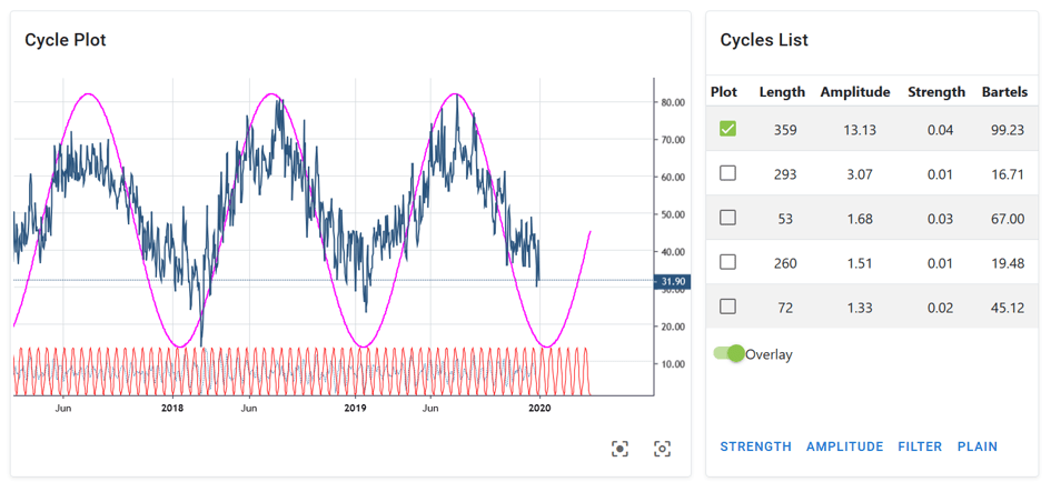

Figure 1: Local temperature Hamburg Germany, Dominant Cycle Length: 359 days, Source: https://cycle.tools (Jan. 2020)
The cycle detection analyzed the dataset and provides us with useful information about the underlying active cycles in this dataset. For the daytime temperature this may be obvious to any eye anyway, but should serve as an introductory example. There are three important structures that have to be identified by any cycle detection engine:
1)
- Which cycles are active in this
dataset?data2)set? - How long are the active dominant cycles?
- Where is the high/low of these cycles aligned on the time scale?
3)
Any cycle detection algorithm must output this information from the analyzed raw data set. In our case, the information is displayed on the right side of the graph as a “cycle list”. It provides an answer to the first question, namely which cycles are currently active, with the most active cycle being plotted at the top of the list. We can identify the most dominant cycle by its amplitude relative to the other detected cycles. In this case there is only one dominant cycle with an amplitude of 13, followed by the next relevant cycle with an amplitude of about 3. The second cycle’s relative size is too small compared to the first to play an important role. We could therefore skip each of the “smaller” cycles in terms of their amplitude compared to the highest ranking cycle with an amplitude of 13.
To answer the second question, the “lengths” information is displayed. For the highest-ranking cycle we see the length of 359 days. This is nothing other than the annual seasonal cycle for a location in Central Europe. But you can see that the recognition algorithm does actually not know that it is “weather”, but is capable of extracting the length from the raw data for us.
After all, the cycle status is the third important piece of information we need: When have the ups and downs of the cycle with a length of 358 days occurred in the past? In technical terminology, this is called the current phase of the dominant cycle. It is represented by the recorded overlay cycle in which the highs and lows are shown in the output as purple line: The low occurs in January/February, while the highs take place in July of that year.
Using these 3 pieces of information about the dominant cycle, we can start with a prediction: We would expect the next low in early February and the next high in July. The dominant cycle is extended into the future. Well, this is an overly simple example, but it shows that identifying and forecasting cycles will provide useful information for future planning.
So that’s the trump card: Any cycle detection alogrithmalgorithm must provide information about
- a) What are the currently active dominant cycles?
- b) How long is the active cycle?
- c) When are past and future highs / lows?
Allow us to continue and apply this algorithm to the financial data set. Similar to the weather cycle, sentiment cycles are often the driving force behind ups and downs in the major markets.
Understanding the sentiment cycles in financial stress is critical to generating returns in the current market environment. Sentiment cycles influence the movement of financial markets and are directly related to people’s moods. Getting a handle on sentiment cycles in the market would substantially improve one’s trading ability.
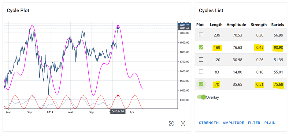
Figure 2 shows the same technique applied to the VIX index, also called the “fear index”. The blue plot is the raw data of the daily VIX data at the time of today’s writing. The detected dominant cycle is shown as an overlay with its length and its phase/time alignment, making it possible to draw the mood cycle into the future.
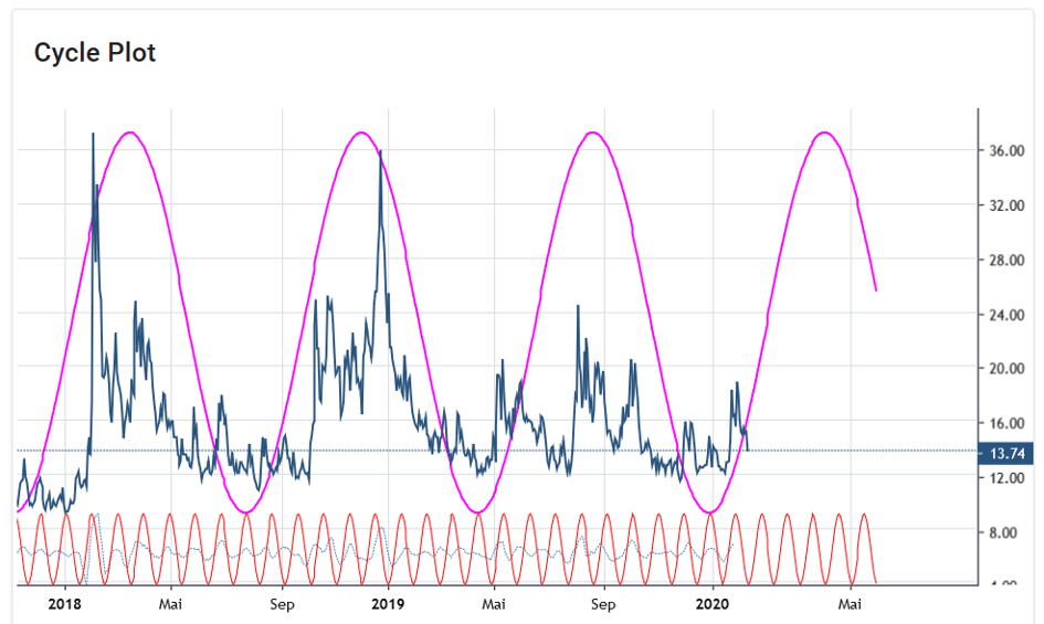

Figure 2: VIX Cycle, Dominant Cycle Length: 180 bars, Source: https://cycle.tools (13. Feb. 2020)
The reading of the VIX sentiment cycles is somewhat different when applied to stock market behavior: Data lows show windows of high confidence in the market and low fear of market participants, which in most cases refer to market highs of stocks and indices. On the other hand, data highs represent a state of high anxiety, which occurs in extreme forms at market lows in particular. Reading the cycle in this way, one would predict a market high that will happen in the current period at the end of December 2019/beginning of 2020 and an expected market low that, according to the VIX cycles, could occur somewhere around April.
Similar to the identification and forecasting of weather/temperature cycles, we can now identify and predict sentiment cycles.
In terms of trading, one should never follow a purely static cycle forecast. The cycle-in-cycles approach should be used to cross-validate different related markets for the underlying active dominant cycles. If these related markets have cyclical synchronicity, the probability for successful trading strategies increases.
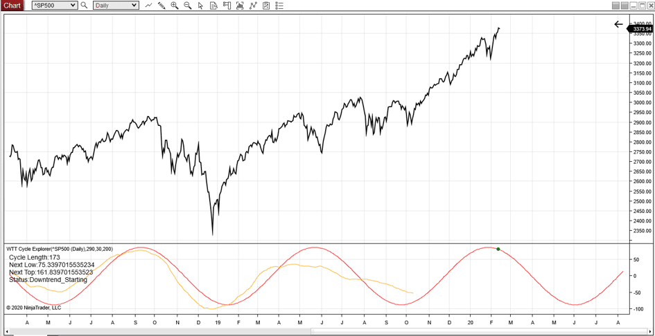
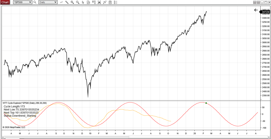
Figure 3 now shows the same method applied to the S&P500 stock market index. The underlying detected cycle has a length of 173 bars and indicates a cycle high at the current time. This predicts a downward trend of the dominant cycle until mid 2020.