Asymmetric Business Cycles and Skew Factors
ThePreface:
Cycle analysis and cycle forecasting often imply the use of a symmetric time distribution between high to low and low to high. This is the underlying framework used by anyone applying mathematical signal processing to cycles and producing cycle-based composite cycle forecasts. This technique is now faced with a new challenge that has emerged over the past 30 years based on financial regulations impacting today’s economic business cycle. The following article will highlight the situation and present the reader with a proposed skew factor to account for this behavior in cycle isforecasting models.
Business cycles are a fundamental concept in macroeconomics. The economy has been characterized by an increasingly negative cyclical asymmetry over the last three decades. Studies show that recessions have become relatively more severe, while recoveries have become smoother, as recently highlighted by Fatas and Mihov. Finally, recessive episodes have become less frequent, suggesting longer expansions.
As a result, booms are increasingly smoother and longer-lasting than recessions.
These characteristics have led to an increasingly negative distortion of the business cycle in recent decades. An extensiveExtensive literature has examined in detail the statistical properties of this empirical regularity and confirmed that the extent of contractions tends to be sharper and faster than that of expansions.
In explanationa ofpaper thispublished in the American Economic Journal on Jan. 2020, Jensen et al. summarized:
Booms become progressively smoother and more prolonged than busts. Finally, in line with recent empirical evidence, financially driven expansions lead to deeper contractions, as compared with equally sized nonfinancial expansions.
When recessions become faster and more severe and recoveries softer and longer, standard symmetric cycle models are doomed to fail. This new pattern presents a challenge tochallenges the existing standardstandard, symmetricsymmetrical, 2-phase cycle models.
Since theory2-phase cycle models are based on a time-symmetric distribution of dominant cycles with mathematical sine-based counting modes from low to low or high to high. However, these models lose their forecasting ability under the assumption that a uniform distribution from high to low and low to high is neededno tolonger copegiven.
A this.new Formodel thisis purpose,needed. we design and estimate aA dynamic skew cycle model that includes a skew factor.
Before introducing a new mathematical model to account for the asymmetric behavior, the cycle difference will be visualized and compared with some diagrams. The following illustration shows on the left side a classical, symmetrical 2-phase cycle on the left (green). Anand asymmetricalan asymmetric 3-phase cycle (red) is highlighted on the right side.(red).
Asymmetric Cycle Model
ForThis modellingfollowing model shown in Chart 1 uses a simplified formula is used, whichthat allows different distortions of the phases with a skew factorfactor, but at the same timealso keeps the length of the whole cycle, from peak to peak, the same without distortion.
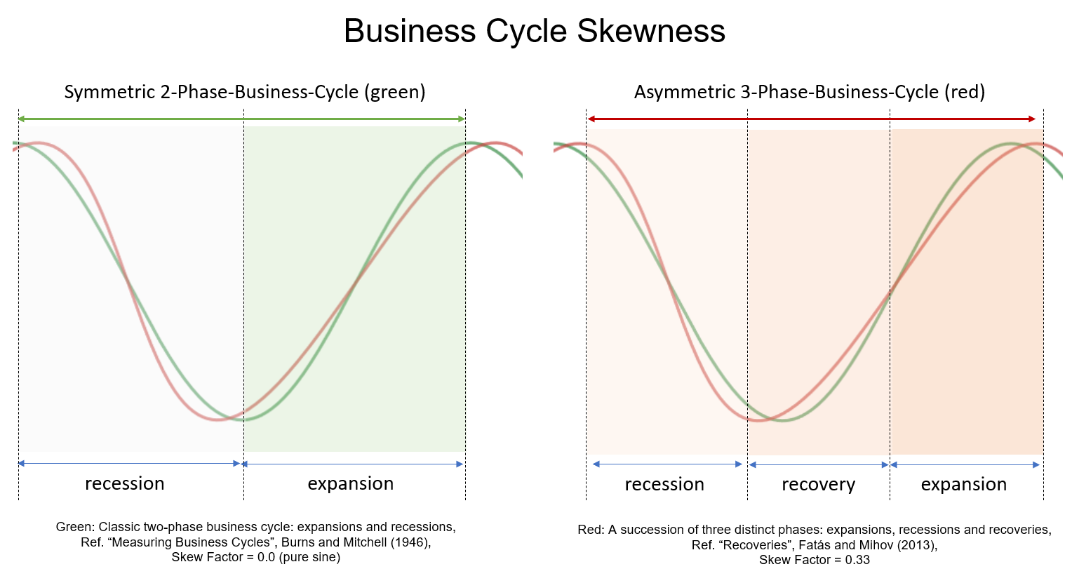
Chart 1: Comparing 2-phase symmetric (green) and 3-phase asymmetric cycle models (red)
The new “skew factor of 0.33factor” used in the red model shows that the upswing phase is twice as long as the recession, while ensuring the same total duration and amplitude of the standardstandard, 2-phase cycle model (green)green, left). This allows us to transfermodel identified cycle lengths and strengths toin the 3-phase model (red, right).
So, if we add the “skew factor” to the traditional mathematical cycle algorithms, we get cycle models that consider the asymmetric changes mentioned above. And thus, the cycle models can be used again for modeling.forecasts.
AExample: hands-The skew factor on example
the S&P 500 index
The firstnext chart 2 shows a detected dominantdominant, symmetric cycle with a length of 175 bars in January 2020,2020 for the S&P 500 index. The light blue price data were not known to the cycle detection algorithm and represent the forecast out-of-sample range. The cycle is shown as a pink overlay. This symmetrical cycle forecast predictedpredicts that the peak would occur as early as the end of 20192019, and thea new low for this cycle to occur in May. As can be seen, the peak was predicted too early and the low too late.
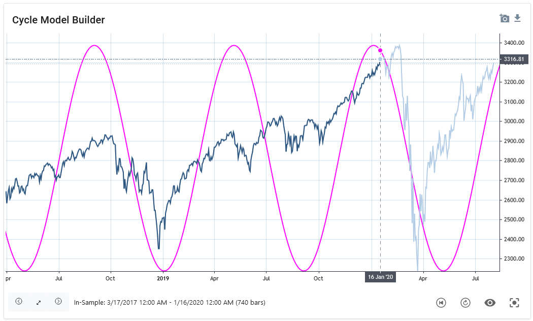
Chart:Chart 2: S&P 500 with 175 day symmetric cycle, skew factor: 0.0, date of analysis: 16. Jan 2020
Now,As ifcan be seen, the predicted high was too early than the real market top, and the predicted low was too late compared to the market low. This is a common observation when using symmetric cycle models in today’s markets. On the one hand, the analyst can now anticipate, based on knowledge of asymmetric variation, that the predicted high will be too early and the plotted low too late. However, additional knowledge of the analyst is required without being represented in the model. A better approach would be to include this knowledge already in the modeling of the cycle projection.
Therefore, we applynow add the skew factor to the detected cycle analysis approach.
In the next graph (Chart 3), a skew factor to the same 175-day cycle, thiscycle is shown in the second graph.applied. The date of analysis is still January 1616, and the light blue is the prediction out-of-sample period. NowHere the asymmetric cycle forecast is able to projectprojects the peak for late January and the expected low for March 2020. Now theThe real price followed this asymmetric cycle projection more accurately.
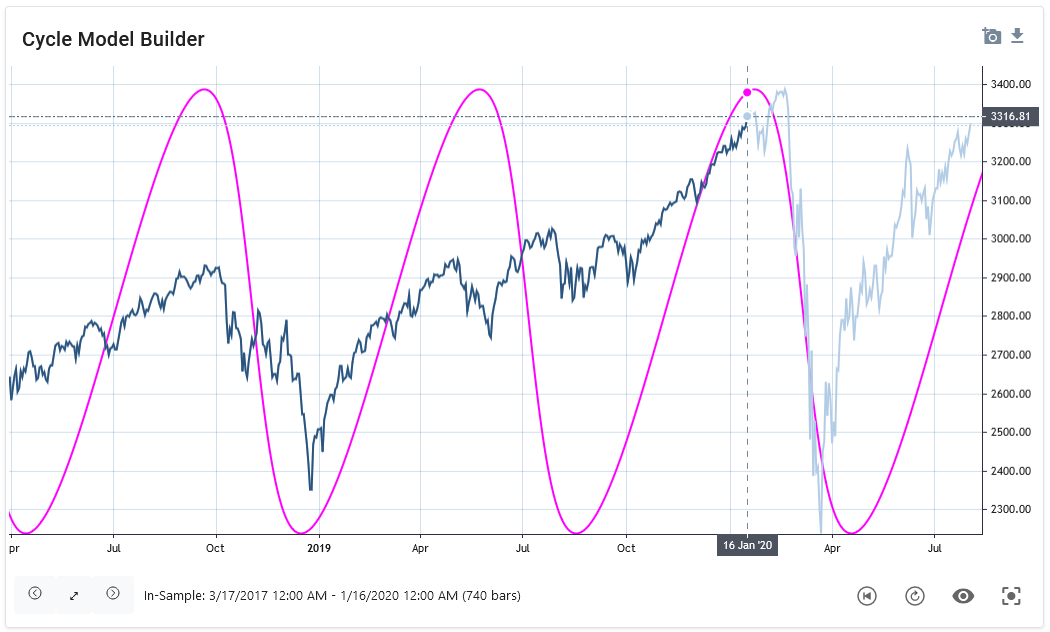
Chart:Chart 3: S&P 500 with 175 day asymmetric cycle, skew factor: 0.4, date of analysis: 16. Jan 2020
This example demonstrates the importance to adapt traditional cycle prediction models with the addition of a skew factor. The introduction of a skew factor is based on the current scientific knowledge of the changed, asymmetric business cycle behavior.
The next paragraph explains how this asymmetry can be applied to existing, mathematical cycle models by introducing the skew factor formula.
Cycle Skew
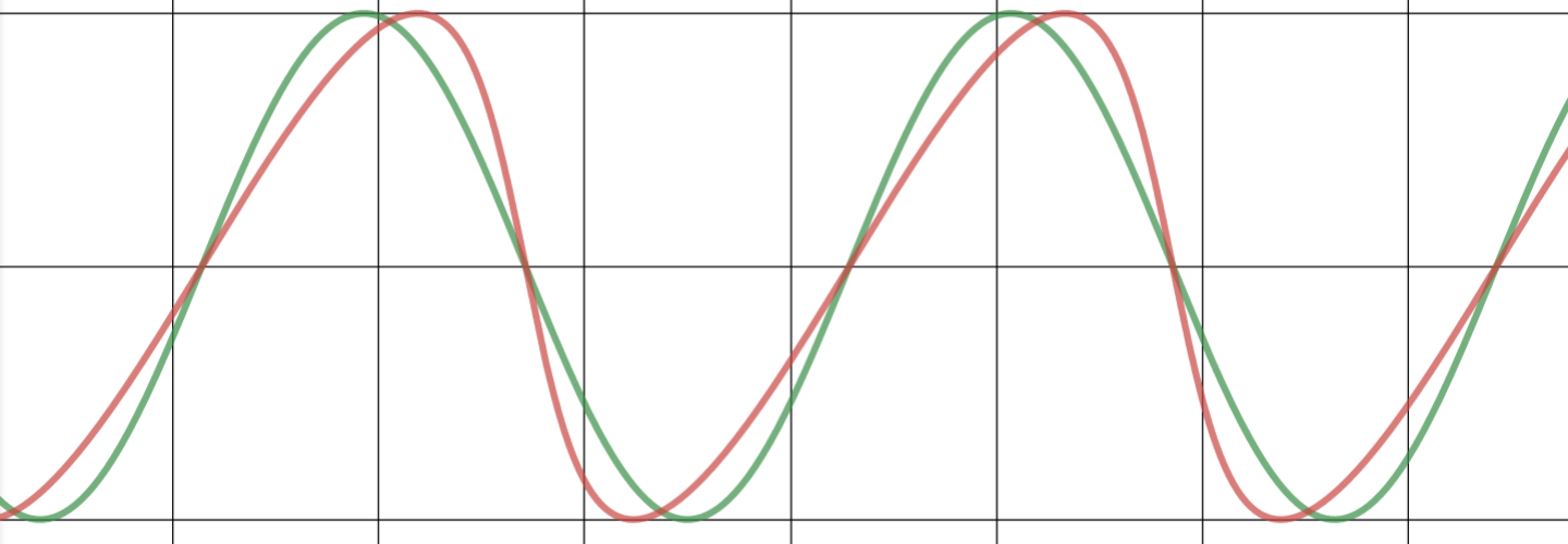
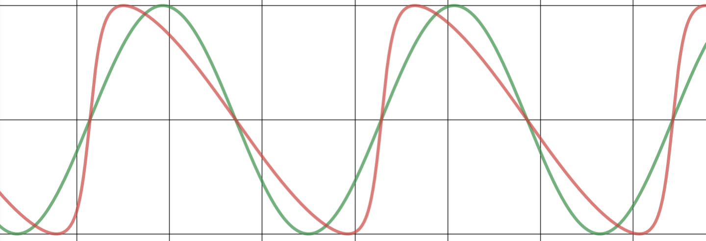
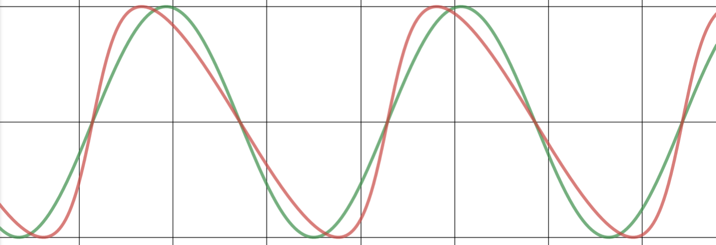
The introduced 'skew factor'factor allows the representation of an asymmetric shape for business cycles in a cyclic modelmodel, as shown in the following examples. The green cycle is a standard sine-wave cycle (skew=0.0); compared to a skewedthe red cycle model withapplies a specific skew factor.
Examples
|
|
 |
|
skew = 0.5 |
skew = 0.75 |
|
|
 |
|
skew = -0.5 |
skew = -0.75 |
(a+cosx)cosn+bsinxsinn(a+cosx)2+(bsinx)2
Desmos interactive playbook: https://www.desmos.com/calculator/ejq06faf93
Math & Code
Equation
To apply the cycle skew, the skewed sine wave equation is introduced instead of a pure sine wave, sin(x), formula:
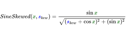
Where:
skew = skew factor [Range: -1 ... +1]
x = phase (rad)
Math LaTeX code
SineSkewed({\color{DarkGreen} x}, {\color{Blue} s_{kew}})=\frac{\sin {\color{DarkGreen} x}}{\sqrt{({\color{Blue} s_{kew}}+\cos {\color{DarkGreen} x})^2+(\sin {\color{DarkGreen} x})^2}}
.NET C# code
Skewed sine wave function
double MathSineSkewed(double x, double skew)
{
  double skewedCycle = Math.Sin(x) /
                       Math.Sqrt(Math.Pow((skew + Math.Cos(x)), 2) + Math.Pow((Math.Sin(x)), 2));

  return skewedCycle;
}
How to use in a cycle forecast algorithm
A common approach is to build cycle prediction models based on detected or predefined values for cycle length, phase, and amplitude. These models use a standard sine wave function to create a cycle forecast or composite forecast projection. To retain these models and not recreate an existing model, the proposal presented in this paper is to simply replace the existing standard sine wave function with the new skewed sine wave function. Thus, any cycle prediction algorithm can remain as is and use the detected cycles with length, amplitude, and phase as input parameters. At the same time, the projection function is replaced with the new skewed sine function instead of the standard sine function.
The main features of this function in brief:
- It is designed as a drop-in replacement for existing sine or cosine functions used for cycle prediction. It is not necessary to adjust the existing overall model. Simply use this function as a drop-in replacement in an existing algorithm.
- A skew factor of 0.3-0.4 should be used to fit the model according to current scientific evidence on the asymmetry of the business cycle.
- The cycle will not be skewed. The length is preserved. Thus, the top-to-bottom and bottom-to-top cycle counts are preserved and are not distorted. The amplitude will not be distorted either. In this way, it is a safe replacement, with the main cycle parameters of length and amplitude remaining intact.
Summary
The current scientific literature shows the increasingly asymmetric behavior of economic cycles. Explanations can be found in the changing behavior of the financial systems in the US and G7 countries. Against this background, previous 2-phase symmetric cycle models need to be adjusted. The demonstrated approach of introducing an additional skew factor into existing sinusoidal models can help to better adapt cycle-based forecasts to this situation.
Further Reading
"Salgado et al. (2020): Skewed BusinessCycles" (2020)https://nbloom.people.stanford.edu/sites/g/files/sbiybj4746/f/skewness_0.pdfCycles"Morley, Piger (2012): The Asymmetric BusinessCycle" (2012)https://www.mitpressjournals.org/doi/10.1162/REST_a_00169Cycle"Jensen et al., (2020): Leverage and Deepening Business CycleSkewness" (2017)https://web.econ.ku.dk/esantoro/images/Skewness.pdfSkewnessFatas andFatas, Mihov (2013),:"Recoveries"https://www.bostonfed.org/employment2013/papers/Fatas_Mihov_Session7.pdfRecoveries
(a+cosx)cosn+bsinxsinn(a+cosx)2+(bsinx)2