# Dynamic Nature of Cycles
#### Cycles are not static
Dominant Cycles morph over time because of the nature of inner parameters of length and phase. Active Dominant Cycles do not abruptly jump from one length (e.g., 50) to another (e.g., 120). Typically, one dominant cycle will remain active for a longer period and vary around the core parameters. The “genes” of the cycle in terms of length, phase, and amplitude are not fixed and will morph around the dominant mean parameters.
The assumption that cycles are static over time is misleading for forecasting and cycle prediction purposes.
These periodic motions abound both in nature and the man-made world. Examples include a heartbeat or the cyclic movements of planets. Although many real motions are intrinsically repeated, few are perfectly periodic. For example, a walker's stride frequency may vary, and a heart may beat slower or faster.
Once an individual is in a dominant state (such as sitting to write a book), the heartbeat cycle will stabilize at an approximate rate of 85 bpm. However, the exact cycle will not stay static at 85 bpm but will vary +/- 10%. The variance is not considered a new heartbeat cycle at 87 bpm or 83 bpm, but is considered the same dominant, active vibration.
This pattern can be observed in the environment in addition to mathematical equations. Real cyclic motions are not perfectly even; the period varies slightly from one cycle to the next because of changing physical environmental factors.
Steve Puetz, a well known cycle researcher, calles this “*Period variability*“:
> “Period variability – Many natural cycles exhibit considerable variation between repetitions. For instance, the sunspot cycle has an average period of ∼10.75-yr. However, over the past 300 years, individual cycles varied from 9-yr to 14-yr. Many other natural cycles exhibit similar variation around mean periods.” *Puetz (2014): in Chaos, Solitons & Fractals*
This dynamic behavior is also valid for most data-series which are based on real-world cycles.However, anticipating current values for length and cycle offset in real time is crucial to identifying the next turn. It requires an awareness of the active dominant cycle parameter and requires the ability to verify and track the real current status and dynamic variations that facilitate projection of the next significant event.
Figures 1 to 3 provide a step-by-step illustration of these effects. The illustrations show a grey static cycle. The variation dynamic in the cycle is represented by the red one with parameters that morph slightly over time. The marked points A to D represent the deviation between the ideal static and the dynamic cycle.
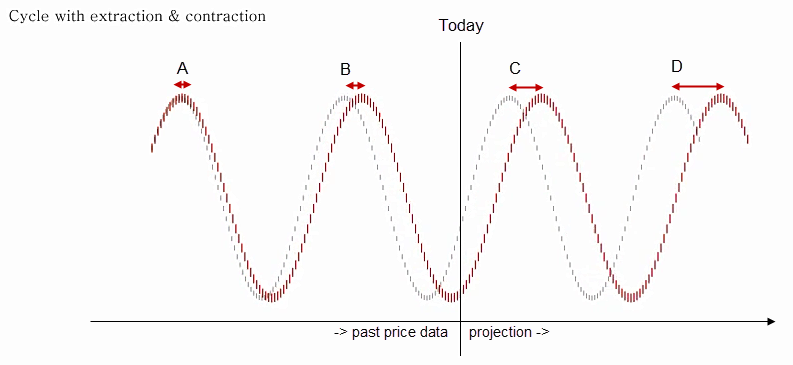
#### Effect A: Shifts in Cycle Length
The first effect is contraction and extraction of cycles, or the “cycle breath.” Possible cycles are detected from the available data on the left side of the chart. Points A and B show an acceptable fit between both cycles. However, the red dynamic cycle has a greater parameter length. The past data reveal that this is not significant, and there is a good fit for the theoretical static and the dynamic cycle at point A and B. Unfortunately, the future projection area on the right side of the chart where trading takes place reflects an increasing deviation between the static and dynamic cycle. The difference between the static and dynamic cycle at points C and D is now relatively high.
[](https://docs.cycle.tools/uploads/images/gallery/2020-05/Cycle_Length_Phase_Shifts.png)
The real “dynamic” cycle has a parameter with a slightly greater length. The consequence is that future deviations increase even when the deviations between the theoretical and real cycle are not visible in the area of analysis. These differences are crucial for trading. As trading occurs on the right side of the chart, the core parameters now and for the next expected cycle turn must be detected. A perfect fit of past data or a two-year projection is not a concern. The priority is the here and now, not a mathematical fit with the past. Current market turns must be in sync with the dynamic cycle to detect the next turn.
Therefore, just as an individual heartbeat cycle approximates a core number, the cycle length will vary around the dominant parameter +/- 5%. Following only the theoretical static cycle will not provide information concerning the next anticipated turning points. However, this is not the only effect.
**Animated Video - Length Shifts:**
---
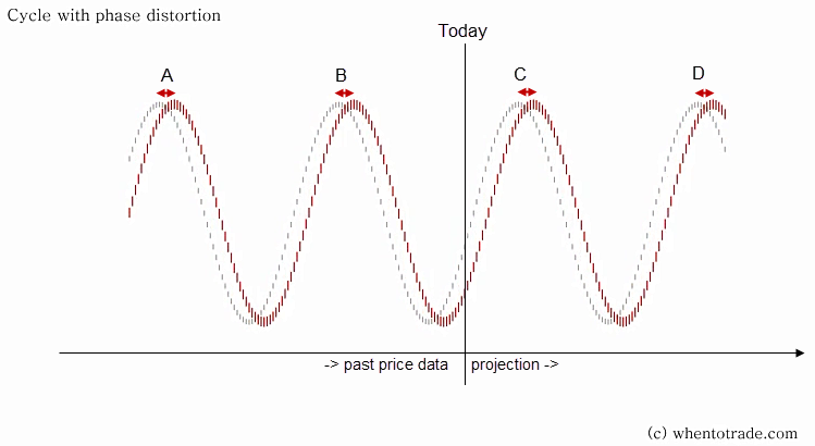
#### Effect B: Shifts in Cycle Phase
The next effect is “offset shifts.” In this case, the cycle length parameter is the same between the static theoretical and the dynamic cycle. The dynamic cycle at point A presents a slight offset shift at the top. In mathematical terms, the phase parameter has morphed. This effect remains fixed into the future. A static deviation is observed between the highs and the lows.
[](https://docs.cycle.tools/uploads/images/gallery/2020-05/Cycle_Length_Phase_Shifts_a.png)
Although this is not a one-time effect, the phase of the dominant cycle will also change continuously by +/- 5% around the core dominant parameters.
**Animated Video - Phase Shifts:**
---
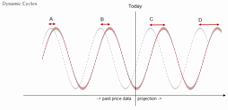
#### The Combined Effects
In practice, both effects occur in parallel and change continuously around the core dominant parameters. Figure 3 presents a snapshot of both effects with the theoretical and the dynamic cycle. The deviation in the projection area at points C and D shows that just following the static theoretical cycle will rapidly become worthless.
[](https://docs.cycle.tools/uploads/images/gallery/2020-05/Cycle_Combined_Shifts.png)
The deviation is to the extent that, at point D, a cycle high is expected for the theoretical static cycle (grey) while the real dynamic cycle (red) remains low at point D.
These two effects occur in a continuous manner. Although the alignment in the past (points A and B) appear acceptable between the static and dynamic cycle, the deviation in the projection area (points C and D) is so high that trading the static cycle will lead to failure.
**Animated Video - Combined Effects:**
****
A cycle forecasting example incorporating these effects explains the consequences on the right side of the chart.
We check the following two examples named “A” and “B”. The price chart is the same for both examples and is represented by a black line on the chart. In both examples, a dominant cycle is detected (red cycle plot) and the price is plotted.
In both examples, two variations of the same dominant cycle are detected. The tops and lows show alignment with the price data and two cycle tops and two cycle lows align. This implies that the same dominant cycle is active in both charts. There is one core dominant cycle and the two detected cycles are variations of this same dominant cycle.
Therefore, from an analytical perspective view, both cycles could be considered valid from observations of the available dataset.
[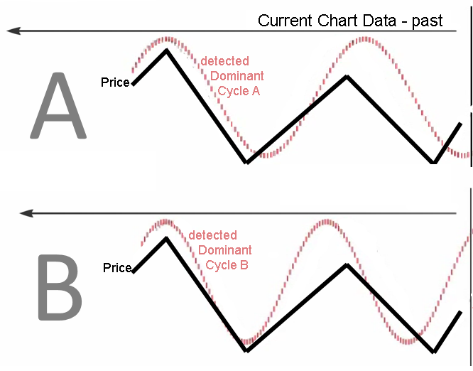](https://docs.cycle.tools/uploads/images/gallery/2020-05/A.png)
The effects reveal that although past data deviation is convincing, it can significantly impact the projection area. We examine the projection of both cycles.
[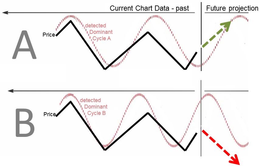](https://docs.cycle.tools/uploads/images/gallery/2020-05/AB2.png)
We observe two contrasting projections. Example A shows a bottoming cycle with a projected upturn to a future top. Example B shows the opposite, a topping out cycle with an expected future downturn.
While we can detect a dominant cycle on the left area of the chart, the detailed dynamic parameters are the significant differentiators and are crucial to a valid and credible projection.
Classic static cycle projections often fail for this reason. Detecting the active dominant cycle represents one part of the process. The second part is to consider the current dynamic parameters with respect to the length and phase of the second part. Although the perfect fit of a cycle within the distant past between price and a static cycle might appear convincing from a mathematical perspective, it is misleading because it ignores the dynamic cycle components. Doing so simplifies the math, but is of no value for trading on the right side of the chart. The examination of past perfect fit static cycles is not necessary. The observance of two to five significant correlations of tops and lows, AND the consideration of current dynamic component updates will yield valid trading cycle projections.
This example underpins the significance of an approach that combines a dominant cycle detection engine with a dynamic component update.
These two effects occur in a continuous manner. Although the alignment in the past (points A and B) appear acceptable between the static and dynamic cycle, the deviation in the projection area (points C and D) is so high that trading the static cycle will lead to failure:
---
#### Video Lesson – Dynamic Cycles Explained
The following video illustrates the two effects in action (6min.)