Cycles Explained

Introduction to Cycles

Cycle Analysis Explained
Cycle Parameters Explained
Dynamic Nature of Cycles
Cycle Playbook
Asymmetric Business Cycles and Skew Factors
Hurst Nominal Cycle Model

Cycle Analysis Explained

Why are cycles so important?

Our daily work schedule is determined by the day and night cycles that come with the rotation of the Earth around its own axis. The orbit of the Moon around the Earth causes the tides of the oceans.

Gardeners have long understood the advantages of working with cycles to ensure successful germination of seeds and high-quality harvest. They work in harmony with the cycles to attain the best results, the best crops.

These are just a few cycles with recurring, dominant conditions that affect all living beings on Earth. So if we are able to recognize the current dominant cycle, we are able to project and predict behavior into the future. Let us start with a simple example to illustrate the power of today’s digital signal processing.

Weather

Figure 1 shows the daily outdoor temperature in Hamburg, Germany (blue). This raw data was fed into a digital signal processor to derive the current underlying dominant cycle and project this cycle into the future (purple).

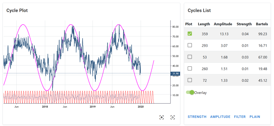
Figure 1: Local temperature Hamburg Germany, Dominant Cycle Length: 359 days, Source: https://cycle.tools (Jan. 2020)

The cycle detection analyzed the dataset and provides us with useful information about the underlying active cycles in this dataset. For the daytime temperature this may be obvious to any eye anyway, but should serve as an introductory example. There are three important structures that have to be identified by any cycle detection engine:

Which cycles are active in this data set?
How long are the active dominant cycles?
Where is the high/low of these cycles aligned on the time scale?

Any cycle detection algorithm must output this information from the analyzed raw data set. In our case, the information is displayed on the right side of the graph as a “cycle list”.

How to sort the active cycles?

The table view at the right part of Figure 1 provides an answer, namely which cycles are currently active, with the most active cycle being plotted at the top of the list. We can identify the most dominant cycle by its amplitude relative to the other detected cycles. In this case there is only one dominant cycle with an amplitude of 13, followed by the next relevant cycle with an amplitude of about 3. The second cycle’s relative size is too small compared to the first to play an important role. We could therefore skip each of the “smaller” cycles in terms of their amplitude compared to the highest ranking cycle with an amplitude of 13.

What is the length of active cycle?

To answer the second question, the “lengths” information is displayed. For the highest-ranking cycle we see the length of 359 days. This is nothing other than the annual seasonal cycle for a location in Central Europe. But you can see that the recognition algorithm does actually not know that it is “weather”, but is capable of extracting the length from the raw data for us.

Where are we in that cycle?

After all, the cycle status is the third important piece of information we need: When have the ups and downs of the cycle with a length of 358 days occurred in the past? In technical terminology, this is called the current phase of the dominant cycle. It is represented by the recorded overlay cycle in which the highs and lows are shown in the output as purple line: The low occurs in January/February, while the highs take place in July of that year.

Using these 3 pieces of information about the dominant cycle, we can start with a prediction: We would expect the next low in early February and the next high in July. The dominant cycle is extended into the future. Well, this is an overly simple example, but it shows that identifying and forecasting cycles will provide useful information for future planning.

So that’s the trump card: Any cycle detection algorithm must provide information about

What are the currently active dominant cycles?
How long is the active cycle?
When are past and future highs / lows?

Sentiment data

Lets continue and apply this algorithm to the financial data set. Similar to the weather cycle, sentiment cycles are often the driving force behind ups and downs in the major markets.

Understanding the sentiment cycles in financial stress is critical to generating returns in the current market environment. Sentiment cycles influence the movement of financial markets and are directly related to people’s moods. Getting a handle on sentiment cycles in the market would substantially improve one’s trading ability.

Figure 2 shows the same technique applied to the VIX index, also called the “fear index”. The blue plot is the raw data of the daily VIX data at the time of today’s writing. The detected dominant cycle is shown as an overlay with its length and its phase/time alignment, making it possible to draw the mood cycle into the future.

Figure 2: VIX Cycle, Dominant Cycle Length: 180 bars, Source: https://cycle.tools (13. Feb. 2020)

The reading of the VIX sentiment cycles is somewhat different when applied to stock market behavior: Data lows show windows of high confidence in the market and low fear of market participants, which in most cases refer to market highs of stocks and indices. On the other hand, data highs represent a state of high anxiety, which occurs in extreme forms at market lows in particular.

Reading the cycle in this way, one would predict a market high that will happen in the current period at the end of December 2019/beginning of 2020 and an expected market low that, according to the VIX cycles, could occur somewhere around April.

Similar to the identification and forecasting of weather/temperature cycles, we can now identify and predict sentiment cycles.

In terms of trading, one should never follow a purely static cycle forecast. The cycle-in-cycles approach should be used to cross-validate different related markets for the underlying active dominant cycles. If these related markets have cyclical synchronicity, the probability for successful trading strategies increases.

Global stock markets

Figure 3 now shows the same method applied to the S&P500 stock market index. The underlying detected cycle has a length of 173 bars and indicates a cycle high at the current time. This predicts a downward trend of the dominant cycle until mid 2020.

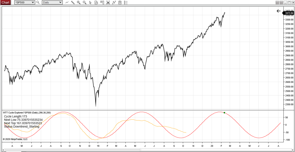
Figure 3: SP500, Dominant Cycle Length: 173 bars, Source: https://cycle.tools API / NT8 (13. Feb. 2020)

We have now discovered two linked cycles, a sentiment cycle with a length of about 180 bars, which indicates a low stress level in December 2019 with an indicative rising anxiety level. And a dominant S&P500 cycle, which leads a market with an expected downtrend until summer 2020. Both cycles are synchronous and parallel in length, timing and direction. This is the key information of a cycle analysis: Synchronous cycles in different data sets that could indicate a trend reversal for the market under investigation.

Well, we can go one step further now. Since more and more dominant cycles are active, you should also look at the 2-3 dominant cycles in a composite cycle diagram.

A composite cycle forecast

Figure 4 shows this idea when analyzing the active cycles for the Amazon stock price. See the list on the right for the current active cycles identified. The most interesting ones have been marked with the length of 169 bars and 70 bars. It is possible to select the most important ones based on the cycle Strength information and the Bartels Score. Not going into the details for these two mathematical parameters, let us simply select the two highest ones for the example. Now, instead of simply drawing the dominant cycle into the future, instead we use both selected dominant cycles for the overlay composite cycle display (purple) which is also extended in the unknown future.

Figure 4: Amazon Stock, Dominant Cycle Length: 169 & 70 bars, Source: https://cycle.tools (04. Feb. 2020)

The purple line shows the cycles with the length of 169 and 70 as well as their detected phase and time alignment in a composite representation. A composite plot is a summary of the detected cycles adding their phase and amplitude at a given time. One can see how well these two cycles in particular can explain the most important stock price movements at Amazon in the last 2 years.

It is interesting to note in this case that a similar composite cycle in Amazon stock price, as previously shown by Sentiment and the S&P500 index cycle, indicates a cyclical downtrend from January to summer 2020.

By combining different data sets and the analysis of the dominant cycle, we can detect a cyclical synchronicity between different markets and their dominant cycles.

The mathematical parameters of cycles allow us to project a kind of “window into the future”. With a projection of the next expected main turning points of the cycle or composite cycle. This information is valuable when it comes to trading and trading techniques. Especially when you are able to identify similar dominant cycles and composite cycles in related markets which are “in-sync”.

The examples used have been kept simple and fairly static to show the basic use for cycle detection and prediction. The projections obtained must be updated with each new data point. It is therefore essential to not only perform this analysis once, statically, but to update it with each new data point.

Knowing how to use cyclical analysis should be part of any serious trading approach and can increase the probability of successful strategies. Because if a rhythmic oscillation is fairly regular and lasts for a sufficiently long time, it cannot be the result of chance. And the more predictable it becomes.

There is often a lack of simple, user-friendly applications to put this theory into practice. We have to work on spreading this knowledge and its application. Instead of the scientific-mathematical deepening of algorithms.

This theory can be applied to any change on our earth as well as to any change of human beings in order to understand their nature and predictable behavior.

Background Information

How does the shown approach work used in these examples?

The technique applied is based on a digital processing algorithm that does all the hard work and maths to derive the dominant cycle in a way that is useful for the non-technical user.

More information on the cycle scanner framework used for these examples can be found in this chapter.

Cycle Parameters Explained

The following chart summarizes all relevant parameters related to a "perfect" sinewave cyle:

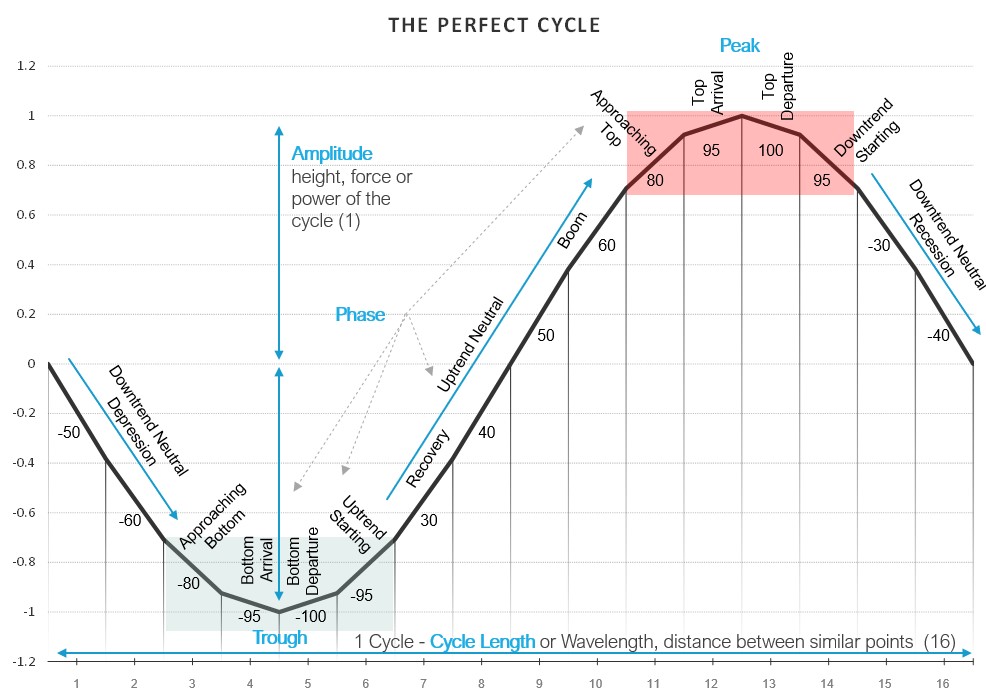
What is Frequency?

Frequency is the number of times a specified event occurs within a specified time interval.
Example:5 cycles in 1 second= 5 Hz

1 cycle in 16 days = 0.0625 cycles/day = 723 nHz

What is Strength?

Strength is the relative amplitude of a given cycle per time interval. (“amplitude per bar”).
Example:
A = 213 , d = 16, s = 13.2 per d

Read more on Cycle Strength in how to "Rank" cycles here.

What is Bartels Score?

The Bartels score provides a direct measure of the likelihood that a given cycle is genuine and not random. It measures the stability of the amplitude and phase of each cycle.

Formula:
B score %= (1-Bartels Value)*100

Range:
0 % : cycle influenced by random events, not significant
100 %: cycle is significant / genuine

Read more on how to validate cycles with the Bartels score here

Dynamic Nature of Cycles

Cycles are not static

Dominant Cycles morph over time because of the nature of inner parameters of length and phase. Active Dominant Cycles do not abruptly jump from one length (e.g., 50) to another (e.g., 120). Typically, one dominant cycle will remain active for a longer period and vary around the core parameters. The “genes” of the cycle in terms of length, phase, and amplitude are not fixed and will morph around the dominant mean parameters.

The assumption that cycles are static over time is misleading for forecasting and cycle prediction purposes.

These periodic motions abound both in nature and the man-made world. Examples include a heartbeat or the cyclic movements of planets. Although many real motions are intrinsically repeated, few are perfectly periodic. For example, a walker's stride frequency may vary, and a heart may beat slower or faster.

Once an individual is in a dominant state (such as sitting to write a book), the heartbeat cycle will stabilize at an approximate rate of 85 bpm. However, the exact cycle will not stay static at 85 bpm but will vary +/- 10%. The variance is not considered a new heartbeat cycle at 87 bpm or 83 bpm, but is considered the same dominant, active vibration.

This pattern can be observed in the environment in addition to mathematical equations. Real cyclic motions are not perfectly even; the period varies slightly from one cycle to the next because of changing physical environmental factors.

Steve Puetz, a well known cycle researcher, calles this “Period variability“:

“Period variability – Many natural cycles exhibit considerable variation between repetitions. For instance, the sunspot cycle has an average period of ∼10.75-yr. However, over the past 300 years, individual cycles varied from 9-yr to 14-yr. Many other natural cycles exhibit similar variation around mean periods.” Puetz (2014): in Chaos, Solitons & Fractals

This dynamic behavior is also valid for most data-series which are based on real-world cycles.However, anticipating current values for length and cycle offset in real time is crucial to identifying the next turn. It requires an awareness of the active dominant cycle parameter and requires the ability to verify and track the real current status and dynamic variations that facilitate projection of the next significant event.

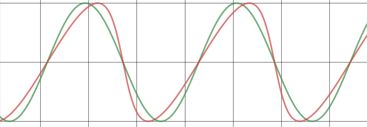
Figures 1 to 3 provide a step-by-step illustration of these effects. The illustrations show a grey static cycle. The variation dynamic in the cycle is represented by the red one with parameters that morph slightly over time. The marked points A to D represent the deviation between the ideal static and the dynamic cycle.

Effect A: Shifts in Cycle Length

The first effect is contraction and extraction of cycles, or the “cycle breath.” Possible cycles are detected from the available data on the left side of the chart. Points A and B show an acceptable fit between both cycles. However, the red dynamic cycle has a greater parameter length. The past data reveal that this is not significant, and there is a good fit for the theoretical static and the dynamic cycle at point A and B. Unfortunately, the future projection area on the right side of the chart where trading takes place reflects an increasing deviation between the static and dynamic cycle. The difference between the static and dynamic cycle at points C and D is now relatively high.

The real “dynamic” cycle has a parameter with a slightly greater length. The consequence is that future deviations increase even when the deviations between the theoretical and real cycle are not visible in the area of analysis. These differences are crucial for trading. As trading occurs on the right side of the chart, the core parameters now and for the next expected cycle turn must be detected. A perfect fit of past data or a two-year projection is not a concern. The priority is the here and now, not a mathematical fit with the past. Current market turns must be in sync with the dynamic cycle to detect the next turn.

Therefore, just as an individual heartbeat cycle approximates a core number, the cycle length will vary around the dominant parameter +/- 5%. Following only the theoretical static cycle will not provide information concerning the next anticipated turning points. However, this is not the only effect.

Animated Video - Length Shifts:

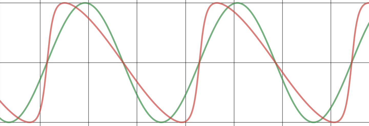
Effect B: Shifts in Cycle Phase

The next effect is “offset shifts.” In this case, the cycle length parameter is the same between the static theoretical and the dynamic cycle. The dynamic cycle at point A presents a slight offset shift at the top. In mathematical terms, the phase parameter has morphed. This effect remains fixed into the future. A static deviation is observed between the highs and the lows.

Although this is not a one-time effect, the phase of the dominant cycle will also change continuously by +/- 5% around the core dominant parameters.

Animated Video - Phase Shifts:

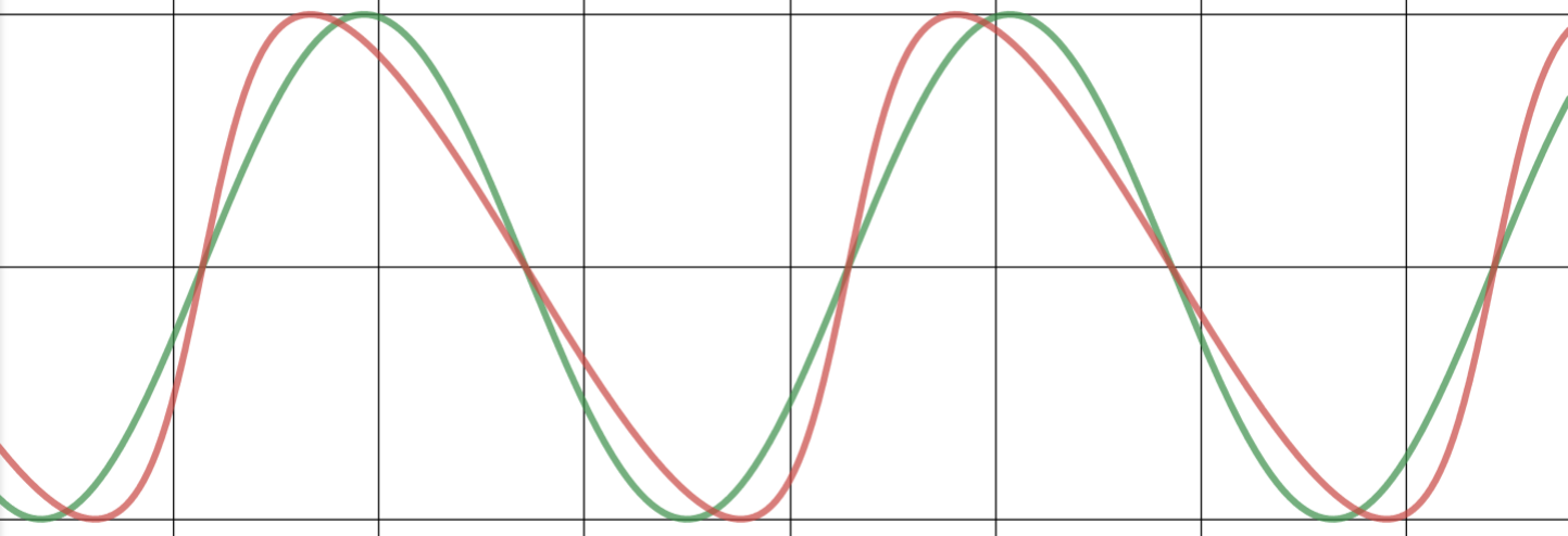
The Combined Effects

In practice, both effects occur in parallel and change continuously around the core dominant parameters. Figure 3 presents a snapshot of both effects with the theoretical and the dynamic cycle. The deviation in the projection area at points C and D shows that just following the static theoretical cycle will rapidly become worthless.

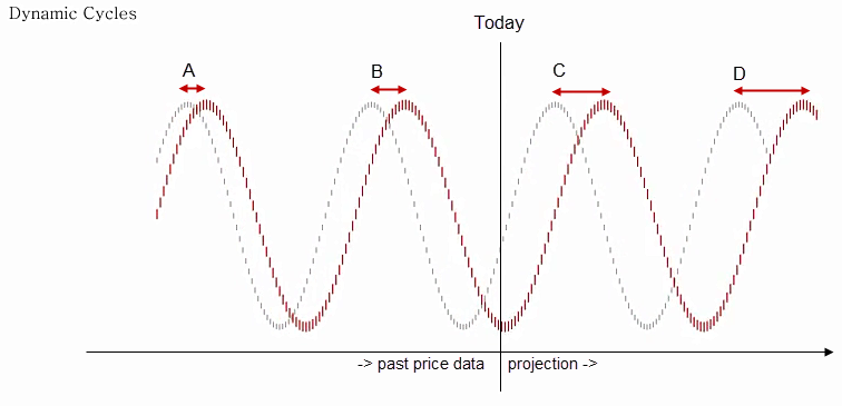
The deviation is to the extent that, at point D, a cycle high is expected for the theoretical static cycle (grey) while the real dynamic cycle (red) remains low at point D.

These two effects occur in a continuous manner. Although the alignment in the past (points A and B) appear acceptable between the static and dynamic cycle, the deviation in the projection area (points C and D) is so high that trading the static cycle will lead to failure.

Animated Video - Combined Effects:

A cycle forecasting example incorporating these effects explains the consequences on the right side of the chart.

We check the following two examples named “A” and “B”. The price chart is the same for both examples and is represented by a black line on the chart. In both examples, a dominant cycle is detected (red cycle plot) and the price is plotted.

In both examples, two variations of the same dominant cycle are detected. The tops and lows show alignment with the price data and two cycle tops and two cycle lows align. This implies that the same dominant cycle is active in both charts. There is one core dominant cycle and the two detected cycles are variations of this same dominant cycle.

Therefore, from an analytical perspective view, both cycles could be considered valid from observations of the available dataset.

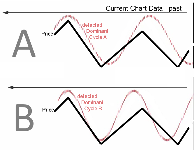
The effects reveal that although past data deviation is convincing, it can significantly impact the projection area. We examine the projection of both cycles.

We observe two contrasting projections. Example A shows a bottoming cycle with a projected upturn to a future top. Example B shows the opposite, a topping out cycle with an expected future downturn.

While we can detect a dominant cycle on the left area of the chart, the detailed dynamic parameters are the significant differentiators and are crucial to a valid and credible projection.

Classic static cycle projections often fail for this reason. Detecting the active dominant cycle represents one part of the process. The second part is to consider the current dynamic parameters with respect to the length and phase of the second part. Although the perfect fit of a cycle within the distant past between price and a static cycle might appear convincing from a mathematical perspective, it is misleading because it ignores the dynamic cycle components. Doing so simplifies the math, but is of no value for trading on the right side of the chart. The examination of past perfect fit static cycles is not necessary. The observance of two to five significant correlations of tops and lows, AND the consideration of current dynamic component updates will yield valid trading cycle projections.

This example underpins the significance of an approach that combines a dominant cycle detection engine with a dynamic component update.

Video Lesson – Dynamic Cycles Explained

The following video illustrates the two effects in action (6min.)

Cycle Playbook

Please click on the chart below to work with the example on desmos:

Direkt Link: https://www.desmos.com/calculator/qoktq3jboh

Asymmetric Business Cycles and Skew Factors

Preface:
Cycle analysis and cycle forecasting often imply the use of a symmetric time distribution between high to low and low to high. This is the underlying framework used by anyone applying mathematical signal processing to cycles and producing cycle-based composite cycle forecasts. This technique is now faced with a new challenge that has emerged over the past 30 years based on financial regulations impacting today’s economic business cycle. The following article will highlight the situation and present the reader with a proposed skew factor to account for this behavior in cycle forecasting models.

Business cycles are a fundamental concept in macroeconomics. The economy has been characterized by an increasingly negative cyclical asymmetry over the last three decades. Studies show that recessions have become relatively more severe, while recoveries have become smoother, as recently highlighted by Fatas and Mihov. Finally, recessive episodes have become less frequent, suggesting longer expansions.

As a result, booms are increasingly smoother and longer-lasting than recessions.

These characteristics have led to an increasingly negative distortion of the business cycle in recent decades. Extensive literature has examined in detail the statistical properties of this empirical regularity and confirmed that the extent of contractions tends to be sharper and faster than that of expansions.

In a paper published in the American Economic Journal on Jan. 2020, Jensen et al. summarized:

Booms become progressively smoother and more prolonged than busts. Finally, in line with recent empirical evidence, financially driven expansions lead to deeper contractions, as compared with equally sized nonfinancial expansions.

When recessions become faster and more severe and recoveries softer and longer, standard symmetric cycle models are doomed to fail. This new pattern challenges the existing standard, symmetrical, 2-phase cycle models.

Since 2-phase cycle models are based on a time-symmetric distribution of dominant cycles with mathematical sine-based counting modes from low to low or high to high. However, these models lose their forecasting ability under the assumption that a uniform distribution from high to low and low to high is no longer given.

A new model is needed. A dynamic skew cycle model that includes a skew factor.

Before introducing a new mathematical model to account for the asymmetric behavior, the cycle difference will be visualized and compared with some diagrams. The following illustration shows a classical, symmetrical 2-phase cycle on the left (green) and an asymmetric 3-phase cycle is highlighted on the right (red).

Asymmetric Cycle Model

This following model shown in Chart 1 uses a simplified formula that allows different distortions of the phases with a skew factor, but also keeps the length of the whole cycle, from peak to peak, the same without distortion.

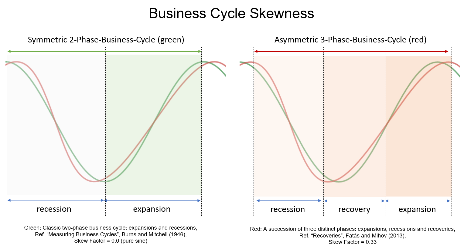
Chart 1: Comparing 2-phase symmetric (green) and 3-phase asymmetric cycle models (red)

The new “skew factor” used in the red model shows that the upswing phase is twice as long as the recession, while ensuring the same total duration and amplitude of the standard, 2-phase cycle model (green, left). This allows us to model identified cycle lengths and strengths in the 3-phase model (red, right).

So, if we add the “skew factor” to the traditional mathematical cycle algorithms, we get cycle models that consider the asymmetric changes mentioned above. And thus, the cycle models can be used again for forecasts.

Example: The skew factor on the S&P 500 index

The next chart 2 shows a detected dominant, symmetric cycle with a length of 175 bars in January 2020 for the S&P 500 index. The light blue price data were not known to the cycle detection algorithm and represent the forecast out-of-sample range. The cycle is shown as a pink overlay. This symmetrical cycle forecast predicts that the peak would occur as early as the end of 2019, and a new low for this cycle to occur in May.

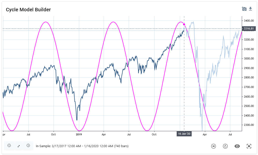
Chart 2: S&P 500 with 175 day symmetric cycle, skew factor: 0.0, date of analysis: 16. Jan 2020

As can be seen, the predicted high was too early than the real market top, and the predicted low was too late compared to the market low. This is a common observation when using symmetric cycle models in today’s markets. On the one hand, the analyst can now anticipate, based on knowledge of asymmetric variation, that the predicted high will be too early and the plotted low too late. However, additional knowledge of the analyst is required without being represented in the model. A better approach would be to include this knowledge already in the modeling of the cycle projection.

Therefore, we now add the skew factor to the detected cycle analysis approach.

In the next graph (Chart 3), a skew factor to the same 175-day cycle is applied. The date of analysis is still January 16, and the light blue is the prediction out-of-sample period. Here the asymmetric cycle forecast projects the peak for late January and the low for March 2020. The real price followed this asymmetric cycle projection more accurately.

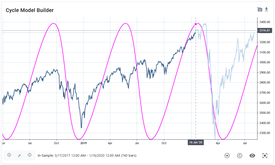
Chart 3: S&P 500 with 175 day asymmetric cycle, skew factor: 0.4, date of analysis: 16. Jan 2020

This example demonstrates the importance to adapt traditional cycle prediction models with the addition of a skew factor. The introduction of a skew factor is based on the current scientific knowledge of the changed, asymmetric business cycle behavior.

The next paragraph explains how this asymmetry can be applied to existing, mathematical cycle models by introducing the skew factor formula.

Cycle Skew

The skew factor allows the representation of an asymmetric shape for business cycles in a cyclic model, as shown in the following examples. The green cycle is a standard sine-wave cycle (s_kew=0.0); the red cycle applies a specific skew factor.

Examples


s_kew = 0.5	s_kew = 0.75


s_kew = -0.5	s_kew = -0.75

$\frac{(a + \cos x) \cos n + b \sin x \sin n}{\sqrt{(a + \cos x)^{2} + {(b \sin x)}^{2}}}$

Desmos interactive playbook: https://www.desmos.com/calculator/ejq06faf93

Math & Code

Equation

To apply the cycle skew, the skewed sine wave equation is introduced instead of a pure sine wave, sin(x), formula:

Where:

s_kew = skew factor [Range: -1 ... +1]
x = phase (rad)

Math LaTeX code

SineSkewed({\color{DarkGreen} x}, {\color{Blue} s_{kew}})=\frac{\sin {\color{DarkGreen} x}}{\sqrt{({\color{Blue} s_{kew}}+\cos {\color{DarkGreen} x})^2+(\sin {\color{DarkGreen} x})^2}}

.NET C# code

Skewed sine wave function

double MathSineSkewed(double x, double skew)
{
  double skewedCycle = Math.Sin(x) / 
                       Math.Sqrt(Math.Pow((skew + Math.Cos(x)), 2) + Math.Pow((Math.Sin(x)), 2));

  return skewedCycle;
}

How to use in a cycle forecast algorithm

A common approach is to build cycle prediction models based on detected or predefined values for cycle length, phase, and amplitude. These models use a standard sine wave function to create a cycle forecast or composite forecast projection. To retain these models and not recreate an existing model, the proposal presented in this paper is to simply replace the existing standard sine wave function with the new skewed sine wave function. Thus, any cycle prediction algorithm can remain as is and use the detected cycles with length, amplitude, and phase as input parameters. At the same time, the projection function is replaced with the new skewed sine function instead of the standard sine function.

The main features of this function in brief:

It is designed as a drop-in replacement for existing sine or cosine functions used for cycle prediction. It is not necessary to adjust the existing overall model. Simply use this function as a drop-in replacement in an existing algorithm.
A skew factor of 0.3-0.4 should be used to fit the model according to current scientific evidence on the asymmetry of the business cycle.
The cycle will not be skewed. The length is preserved. Thus, the top-to-bottom and bottom-to-top cycle counts are preserved and are not distorted. The amplitude will not be distorted either. In this way, it is a safe replacement, with the main cycle parameters of length and amplitude remaining intact.

Summary

The current scientific literature shows the increasingly asymmetric behavior of economic cycles. Explanations can be found in the changing behavior of the financial systems in the US and G7 countries. Against this background, previous 2-phase symmetric cycle models need to be adjusted. The demonstrated approach of introducing an additional skew factor into existing sinusoidal models can help to better adapt cycle-based forecasts to this situation.

Hurst Nominal Cycle Model

Hurst's cycle theory states that the movement of financial market prices is the result of the combination of harmonically related cycles. Hurst recommended a collection of 11 cycles for daily analysis. These cycles are referred to as the Nominal Model.

He did extensive research and discovered 11 cycles ranging from 5 days to 18 years found in a large number of stocks. He published the average wavelength of each of these cycles in his Cycle Course.

Nominal cyclical model is actually the full name, but is simplified to Nominal Model for simplicity. Thus, for example, what we are often referring to is the nominal 20-week cycle, which means that we are discussing the cycle to which the name 20 weeks has been given. The cycle is not really 20 weeks long due to the dynamic nature of cycles. Cycles are not perfectly even. Cycles vary around their length, phase and amplitude over time. Therefore the use of additional techniques to deal with the principle of cycle variation, like Digital Signal Processing, are required.

The Hurst Nominal Cycle Model

Name (Nominal Cycle)	Average length	Average length (days)
5 day	4.3 days	4.3 days
10 day	8.5 days	8.5 days
20 day	17 days	17 days
40 day	34.1 days	34.1 days
80 day	68.2 days	68.2 days
20 week	19.48 weeks	136.4 days
40 week	38.97 weeks	272.8 days
18 month	17.93 months	545.6 days
54 month	53.77 months	1636.8 days
9 year	8.96 years	3272.6 days
18 year	17.93 years	6547.2 days

Source: Hurst Cycles Course

Cycles Explained

Cycle Analysis Explained

Weather

Sentiment data

Global stock markets

A composite cycle forecast

Background Information

Cycle Parameters Explained

What is Frequency?

What is Strength?

What is Bartels Score?

Dynamic Nature of Cycles

Cycles are not static

Effect A: Shifts in Cycle Length

Effect B: Shifts in Cycle Phase

The Combined Effects

Video Lesson – Dynamic Cycles Explained

Cycle Playbook

Asymmetric Business Cycles and Skew Factors

Asymmetric Cycle Model

Example: The skew factor on the S&P 500 index

Cycle Skew

Math & Code

Equation

Math LaTeX code

.NET C# code

How to use in a cycle forecast algorithm

Summary

Further Reading

As published in "Cycles Magazine":

Hurst Nominal Cycle Model

The Hurst Nominal Cycle Model